Drop Down list in Spreadsheet looks more professional. And it helps out to input some data quickly. Google Spreadsheet has an option called “data Validation” which allows us to create a decent drop-down without any coding at all.
Google Sheets drop down list can be set up to manage and enter a lot of data with ease.
It can also be useful to avoid spelling mistakes in the sheets, so that discrepancy in the final calculation can be ignored.
We can use a drop down to track a lot of things, example a status of your work, whether completed, Ongoing or even rejected. Which can be instantly updated.
Google Sheets drop-down looks trendy and the metrics can be maintained effortlessly when you are working with a huge number of teams.
Create a Drop down List in Google Sheets
Step 1. Open a Google Spreadsheet on where you want to create a drop down menu.
For an instance, I had taken a spreadsheet and entered some random data.
Step 2. Enter some data in the next column “H” which you want to be shown in the drop-down menu.
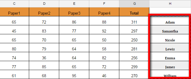
Go through the above image for better insights. (You can add this data to another sheet as well. And if you don’t want to show that information or even hiding that column is possible, here I had added in the same sheet just for the demo).
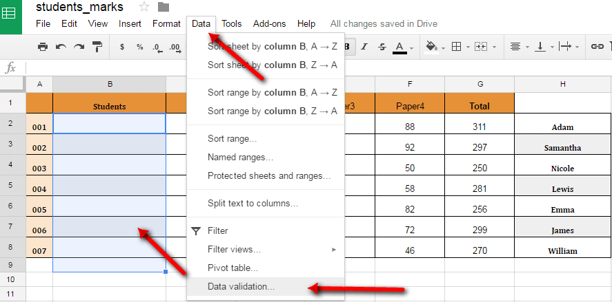
Step 3. Now make the selection where you want the drop down to be created (Refer below image selected Column “B”)
Step 4. Navigate To Data – Data Validation from the menu to create Google sheets drop down, it can also be accessed by right click on the selected area.
Step 5. A pop-window will appear now, asking for some details.
Cell Range: It is basically the range of where the dropdown will be created (leave it the same as it is) as we already made the selection before.
Criteria: There would be some categories in the criteria in drop down list, List from a range, List of items, number, text, data, custom formula. We can select any one of them according to our requirement.
Step 6. Here we are going to create a dropdown list with the selected range, so select the first option “List from the range.”
Step 7. Now Enter the range H2: H in the range column, with the data from which we want to create the drop down list in B column. (Select data range button can also be used to auto select the data, click and drag the desired column fields).
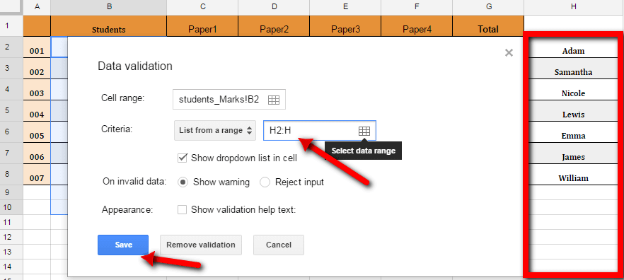
Note: “By selecting H2:H here you had selected the entire column, just in case going forward if we want to add some more data in the same column, which will be automatically get included in the drop-down list. We should do it just to avoid going through this process again and again.
Step 8. Click on “Save” Button.
Step 9.Now you will be able to see the drop down list created for the selected area with the same data or names we have entered.
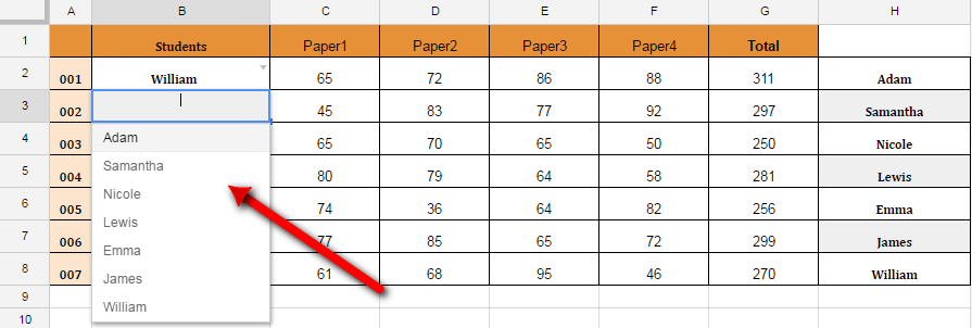
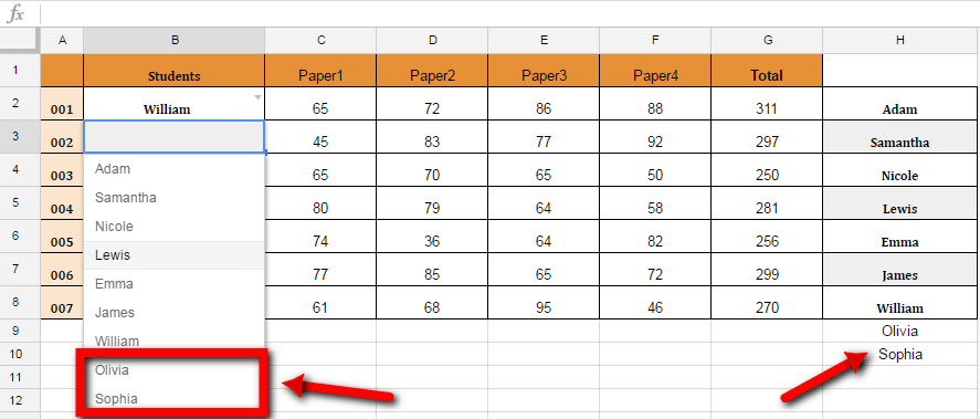
The coolest thing, as mentioned above, whenever we add some data in the H column, same will be reflected in the drop down list.
Check for the below image for better insights earlier Olivia and Sophia names were not there, as we have added in the H column it automatically can be seen in the drop-down list as well.
Manual Process To Create Google Sheet Drop Down List
1. Open Google Spreadsheet, Select a cell and right – click on it
2. Select Data Validation
3. Criteria – List of Items – Enter the data separating with commas
4. Hit Save button, when you are done.
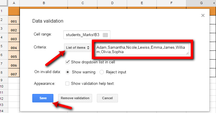
By choosing “List of items” from the Criteria category we can manually enter the names or any other information by separating with commas for creating drop-down list.
Disadvantages creating a drop-down manually – Each time you want to add the data you have to go through the data validation process for the selected columns.
Google Spreadsheets are very robust and useful if used in the proper way. Those can dominate any similar tools present in the market. In fact, if you are well versed with some functions or coding process, you can make use of the Code Editor in it. Tons of functions can be added to do sort the data. And calling the data from the other sheets.